Reveal the Secret Within
This section is for generating Autocorrelation Function (ACF) and Partial Autocorrelation Function (PACF) plots of the time series data. The function acf2 is used here.
No Systematic Trends: Think of it as your data hovering around a roughly constant average value over time. No clear upward or downward drifts.
Variance is Consistent: Your data doesn’t get systematically more ‘spread out’ as time goes on.
Why It Matters: Lots of time series analysis methods, including ARIMA modeling, often perform best when your data is stationary (or you’ve made transformations to achieve this).
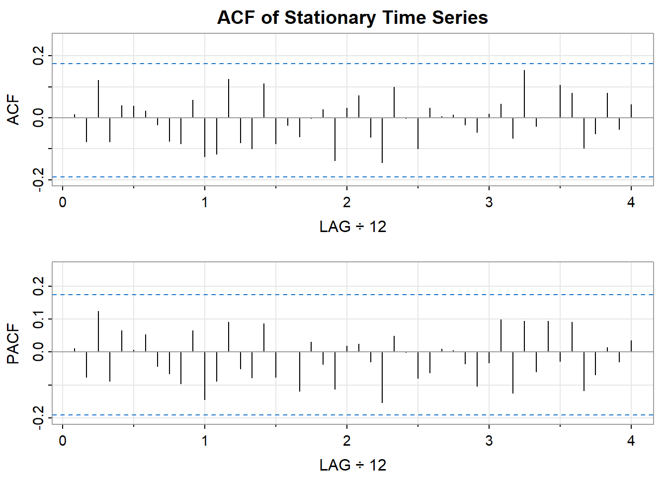
Let’s take a look at the ACF and PACF plots of this series in order to identify the best model for this series.
Interpreting the ACF Plot (acf_stationary)
Significant Spikes: Are there tall bars exceeding the blue dashed lines early on? This implies correlation at specific lags (e.g., today is similar to yesterday).
Decaying Pattern: Does the spike height drop rapidly, with most bars within the dashed lines after a few lags? This is common for stationary series, as further ‘echoes’ in time get fainter.
No Obvious Seasonality: If data had monthly cycles, your ACF would reflect it with repeated spikes every 12 lags. You likely won’t see this here.
What about the PACF?
Other common methods is to use the Box-Ljung test or the Durbin-Watson test. These tests are used to null hypothesis that there is no autocorrelation in the data. If the p-value of the test is less than a certain significance level (e.g., 0.05), then we can reject the null hypothesis and conclude that there is autocorrelation in the data.
Durbin-Watson Test (dwtest): A formal statistical test to detect if there’s significant autocorrelation in the residuals.
Ljung-Box Test (Box.test): The Ljung-Box test checks for autocorrelation in the residuals of a time series model. Autocorrelation here means that the residuals (errors) of the model are correlated with each other at different lags.
Null Hypothesis:
Here are some steps you can take to check for autocorrelation in your time series data:
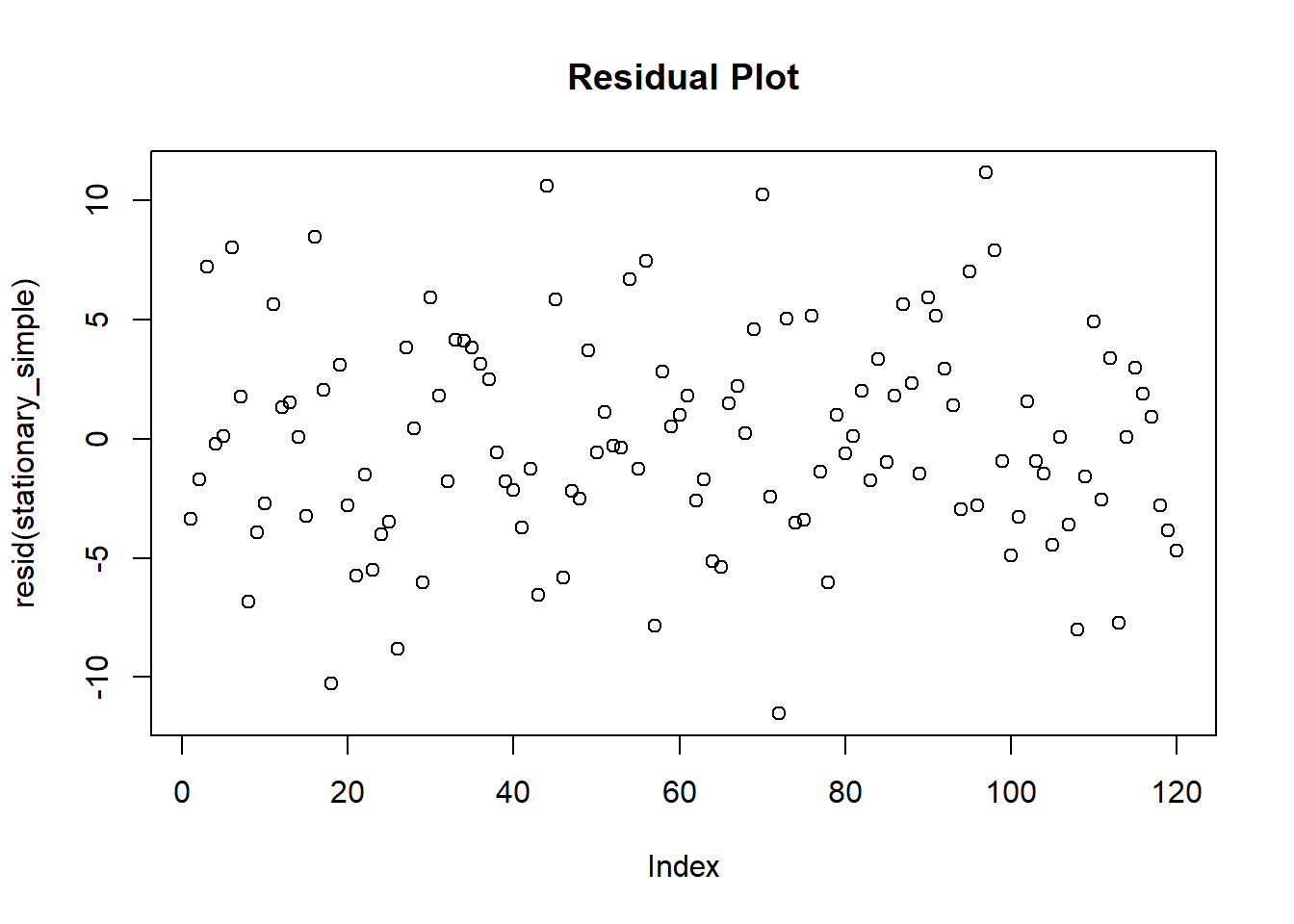
Fit a linear regression model to your data.
Call:
stats::lm(formula = value ~ t, data = stationary_df)

Residuals:
     Min       1Q   Median       3Q      Max
-11.5272  -2.8354  -0.2433   2.9391  11.1638

Coefficients:
             Estimate Std. Error t value            Pr(>|t|)
(Intercept) 50.581625   0.823364  61.433 <0.0000000000000002 ***
t           -0.008337   0.011810  -0.706               0.482
---
Signif. codes:  0 '***' 0.001 '**' 0.01 '*' 0.05 '.' 0.1 ' ' 1

Residual standard error: 4.482 on 118 degrees of freedom
Multiple R-squared:  0.004206,  Adjusted R-squared:  -0.004233
F-statistic: 0.4984 on 1 and 118 DF,  p-value: 0.4816
Calculate the residuals from the model.
Plot the autocorrelation function (ACF) of the residuals.
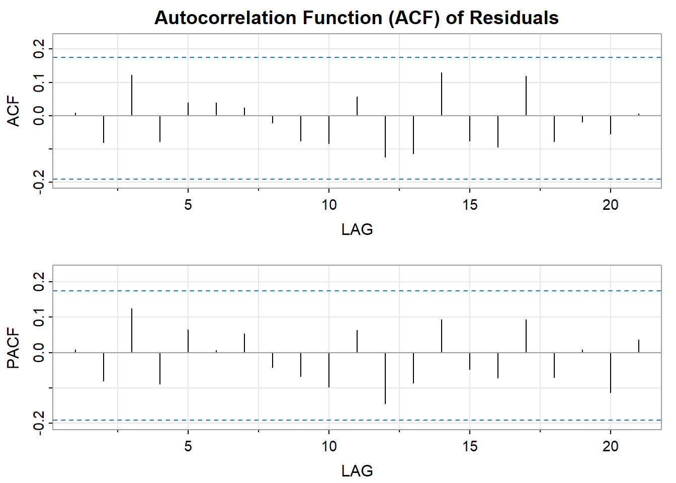
     [,1]  [,2] [,3]  [,4] [,5] [,6] [,7]  [,8]  [,9] [,10] [,11] [,12] [,13]
ACF  0.01 -0.08 0.12 -0.08 0.04 0.04 0.02 -0.02 -0.08 -0.08  0.06 -0.12 -0.11
PACF 0.01 -0.08 0.12 -0.09 0.06 0.01 0.05 -0.04 -0.07 -0.10  0.06 -0.14 -0.09
     [,14] [,15] [,16] [,17] [,18] [,19] [,20] [,21]
ACF   0.13 -0.08 -0.09  0.12 -0.08 -0.02 -0.06  0.01
PACF  0.09 -0.05 -0.07  0.09 -0.07  0.01 -0.11  0.04
Perform a Durbin-Watson test on the residuals.
    Durbin-Watson test

data:  stationary_df$value ~ stationary_df$t
DW = 1.9701, p-value = 0.3979
alternative hypothesis: true autocorrelation is greater than 0In time series analysis, especially when dealing with ARIMA models, the distinction between the autocorrelation in the observed time series and the autocorrelation in the residuals is crucial. A significant part of model validation involves checking for autocorrelation in residuals to ensure the model is appropriately fitted to the data.
The observed time series often has autocorrelation, and that’s expected. The goal of time series modeling is to capture this autocorrelation. Many real time series inherently display autocorrelation. This means that the current value in the series is correlated with its previous values. For instance, today’s temperature is often similar to yesterday’s, or sales in one month might be influenced by sales in the previous months. This autocorrelation is precisely why we use models like ARIMA. These models are designed to capture and explain such autocorrelation in the data.
Accurate Parameter Estimates: Autocorrelation, if present in your data, violates assumptions of standard models like OLS. To get reliable estimates of things like the intervention effect in ITS, you need to account for this dependence between observations over time.
Valid Inference: Statistical tests, p-values, and confidence intervals rely on certain assumptions about errors. Autocorrelation invalidates these, so without modeling it, your conclusions might be incorrect.
The residuals of the model should ideally not be autocorrelated. If they are, it implies that the model has missed some aspect of the data’s structure, and there might be room for improvement in the model. After fitting a time series model like ARIMA, the residuals (the differences between the observed values and the model’s predicted values) should show no autocorrelation.
If residuals are autocorrelated, it suggests that the model has not fully captured all the information in the time series, particularly the patterns or structures related to time. Essentially, it means there’s still some predictable aspect left in the residuals, which should have been accounted for by the model.
Ideal residuals should resemble white noise, meaning they should be random and not exhibit any discernible patterns or trends. This indicates a well-fitting model.
Model Diagnostics: Non-autocorrelated residuals are one indicator of a well-specified model. If autocorrelation remains in the residuals, it suggests that there’s more structure in the data that your model isn’t capturing.
Improved Forecasting: For many time series applications, the goal is forecasting future values. Models that leave autocorrelation in the residuals may produce less accurate forecasts, as they’re not fully understanding the patterns.
Imagine fitting a simple linear regression to estimate the effect of an intervention in ITS. If your time series data exhibits positive autocorrelation (positive values tend to follow other positive values), your standard errors in OLS will be too small, making the intervention effect appear more statistically significant than it potentially is.
Caveats and Nuances:
Sometimes, autocorrelation is merely a symptom of non-stationarity in your time series. In that case, modeling autocorrelation alone won’t solve the problem - you might need differencing or other transformations.
Even with appropriate modeling, sometimes slight residual autocorrelation persists. Statistical tests might flag it, but a trade-off is made between complexity and parsimony.
While the ultimate goal is to identify a model that explains the patterns in your time series thoroughly, we actively model the dependency between values across time to get a valid, reliable model whose residuals behave more in line with statistical assumptions.